

.
BROADBAND SEISMIC OBSERVATIONS AT THE HAWAII-2 OBSERVATORY DURING ODP LEG 200
R. A. STEPHEN1, F. K. DUENNEBIER2, D. Harris2, J. Jolly2, S. T. BOLMER1,
P. BROMIRSKI3, and the ODP Leg 200 Scientific PARTY4
1 Department of Geology
and Geophysics, Woods Hole Oceanographic Institution
2 Department of Geology and Geophysics, University of
Hawaii
3 Center for Coastal Studies, Scripps Institution of Oceanography,
University of California
4 Ocean Drilling Program, Texas A&M University
Abstract
Ocean
Drilling Project Leg 200 was the first leg in deep sea and ocean drilling
history to conduct operations in the vicinity of a continuously operating broadband
seafloor seismometer. In 1998 investigators from the University of Hawaii, Woods
Hole Oceanographic Institution, and Incorporated Institutions for Seismology
had installed a broadband, shallow buried seismometer at the Hawaii-2 Observatory
site [Duennebier et al., 2002] and data was acquired in real time in Oahu over
the Hawaii-2 transoceanic cable. Hole 1224D was drilled, cased and cemented
at the site so that a broadband borehole seismometer could be emplaced in the
future. The noise from the JOIDES Resolution as it approached and left the site
as well as during all on-site operations was acquired continuously in Oahu.
In addition shots with 80 cubic inch water guns during single channel seismic
tests were also recorded in Oahu. The information from the seismic survey will
help to establish the geological environment in the context of other ODP basement
holes, it will provide valuable background information for other geophysical
experiments at the site, and it will provide local structural information to
predict the future performance of the broadband borehole seismometer. This work
was supported by a grant from JOI-USSAC. We would like to thank the Earthquake
Research Institute at the University of Tokyo for a Visiting Professorship for
RAS during which much of this work was carried out. [Duennebier , F.K., D.W.
Harris, J. Jolly, J. Babinec, D. Copson, and K. Stiffel, The Hawaii-2 observatory
seismic system, IEEE Journal of Oceanic Engineering, 27, 212-217, 2002.]
Introduction
Drilling at the H2O site (Figure
1) provides a unique opportunity to observe drilling- related noise from
the JOIDES Resolution and other ambient noise on a seafloor seismometer in the
frequency band of 0.001–60 Hz. The University of Hawaii operates an OBSS
composed of a Guralp CMG-3T three-component broadband seafloor seismometer and
a conventional 4.5-Hz three-axis geophone at H2O [Duennebier et al., 2000; Duennebier
et al., 2002]. The Hawaii-2 Observatory is a cabled, deep sea capability (Figure
2). The drilling activity took place 1.5km northeast of the buried seismometers
(Figure 3). Data are acquired continuously and are made
available to scientists worldwide through the IRIS Data Management Center in
Seattle. The University of Hawaii also maintained a Web site showing seismic
data from H2O during the cruise (www.soest.Hawaii.edu/H2O/).
Unless otherwise indicated all of the data we show
here are from the Guralp CMG-3T three component seismometer in acceleration
units (m/sec^2). All times are given in UTC, which is equal to local time +
9 hr. Occasionally days are represented by the Julian day, the consecutive number
of the day in the year. The objective of this report is to present an overview
of the seismic behavior and some of the natural and man-made noise sources at
the site. For more information on seismic ambient noise levels in the ocean
see Webb [Webb, 1998]; for an introduction to earthquake seismology see Lay
and Wallace [Lay and Wallace, 1995].
At the OSN pilot experiment site in 1998, we deployed
seafloor, buried, and borehole broadband seismometers in order to compare the
performance of different styles of installation. Figures 4
and 5 summarize for vertical and horizontal component data,
respectively, the improvement that we expect to see in ambient seismic noise
on placing a sensor in basement at H2O rather than on or in the sediments. Above
0.3 Hz, the seafloor, buried, and borehole spectra at the OSN-1 site show the
borehole to be 10 dB quieter on vertical components and 30 dB quieter on horizontal
components [Collins et al., 2001; Stephen et al., 2003]. Shear wave resonances
(or Scholte modes) are the physical mechanism responsible for the higher noise
levels in or on the sediment. The resonance peaks are particularly distinct
and strong at the H2O site. By placing a borehole seismometer in basement at
H2O, we expect to eliminate these high ambient noise levels.
Figure 6 shows a vertical
component spectrogram from December 16, 2001 to January 27, 2002 (Julian days
356/2001 to 27/2002). A spectrogram is a display of energy levels as a function
of frequency vs. time. In this case the frequency range of interest is 0.001–60
Hz. In this band, sea state (the gravity waves on the surface of the ocean)
is the dominant source of ambient noise. It has been shown that the microseism
peak, the broad vertical red band at frequencies from 0.2 to 0.3 Hz, is created
by nonlinear wavewave interaction of surface gravity waves [Longuet-Higgins,
1950]. This peak is a ubiquitous feature on all terrestrial seismograms and
is observed at stations deep within the continents. It is interesting to note
that the amplitude of this peak is not dramatically greater for seafloor stations
than for some land stations (Figures 5 and 6).
The thin, constant-frequency red bands near 1.1
and 2.3 Hz in Figure 6 correspond to resonances in the
thin sediment cover at this site [Godin and Chapman, 1999; Zeldenrust and Stephen,
2000]. These bands are another ubiquitous feature observed on seafloor seismometers
either on or in sediment layers. Their frequency will depend on the sediment
thickness and velocity structure local to the station, but for a given station
the frequencies are constant. The resonances are observed as bands in the ambient
noise field and as ringing after impulsive signals. More resonant frequencies
are apparent in the horizontal (x) component spectrogram (Figure
7). A complete explanation for the frequency and relative amplitude of these
resonances is still in progress. The major reason for installing broadband seismometers
in boreholes on the seafloor is to attenuate the effects of these sediment resonances.
Ambient noise spectra from the OSN pilot experiment (Figures 4
and 5) show that these resonances are much more pronounced
on the seafloor and shallow buried sensors than on the borehole sensor.
The spectrograms in Figures 6
and 7 show characteristic "chevron" patterns
about the microseism peaks. On the high frequency side, there are red bands
that slope upward to the left from ~1 to 0.2 Hz over 1.5 to 2 days. They terminate
at the "microseism peak for local sources" near 0.2Hz. (The narrowness
of the peak at 0.2Hz in the vertical component spectra (Figure 4) is reminiscent
of a sediment resonance and there may be multiple processes creating this peak.)
The model for this phenomenon is a steady wind creating local waves. Imagine
the wind blowing steadily over a calm sea. Initially small waves with short
wavelengths and relatively high frequencies are generated by the wind. As the
wind continues to blow the waves get larger, longer in wavelength, and lower
in frequency. Often, the intervals when the JOIDES Resolution was waiting-on-weather
correspond to the later times in the evolution of this noise. The microseism
band is shown with an expanded frequency scale in Figure 8.
The other arms of the chevrons are red bands that slope upward to the right
between 0.1 and 0.2Hz over 2 to 3 days. This is attributed to swell from distant
storms [Babcock et al., 1994; Bromirski and Duennebrier, 2000; Bromirski et
al., 1999].
Whales are a biological seismic source.
Figure 9 shows a sample of a whale song as we arrived at Site 1224 on 26
December. This figure shows a time history of the vertical component of seafloor
acceleration in 30-s segments for 2.5 min near 1550 UTC on 26 December. The
largest-amplitude events are whale songs occurring in wave packets of four wavelets
about once every 30 s. The four wavelets, separated by 3 to 7 s, correspond
to the sound traveling directly from the whale to the seafloor plus multiple
bounces (echoes) of the sound in the water column.
Figure 10 is formatted similarly
to Figure 9 but covers a 25-min time interval. Water gun
arrivals are observed in the first 10 min. The rest of the time series is punctuated
with whale calls, except for the two bands of three traces each shown in red.
A characteristic feature of the whale songs is that they stop every 15 to 20
min while the whale breathes. In this case, the whale sings for 15 min, takes
a breath for 1.5 min, and then repeats the process.
The principal motivation behind drilling at the
H2O is to provide a high-quality seismic station for the Global Seismic Network.
Some small earthquakes did occur while we were on site. A quick and easy way
to scan all of the data continuously is to display root-mean-square (RMS) energy
levels in one-octave bands as a function of time. An example for the vertical
(z) component on 7 January is shown in Figure 11. In this
example, most of the variability during the day is occurring in the octave centered
at 4 Hz. The large peaks near 5 and 20 hr can be identified as T-phases from
earthquakes. Time series and spectra for the event near 21 hr are shown in Figure
12. The event has a duration of ~20 s and has a broad frequency content,
characteristics of T-phases. Note that the energy level of the microseism peak
near 1 Hz does not increase with the arrival. The energy level of the sediment
resonances near 2.8, 4.1, and 5.7 Hz, however, increases by up to 20 dB (a factor
of 10 in amplitude). A second earthquake example is shown in Figure
13. The arrival in this case is spread over a longer time interval, and
there is no detectable energy below the microseism peak.
Shipping is a major man-made source of noise in
the ocean. Figure 14 shows an RMS summary of the vertical
(z) component for 25 December. The RMS level in the octave centered at 8 Hz
increases by 50 dB from 5 to ~12 hr and decreases again at ~15 hr. This event
can also be seen in Figure 6 halfway through 25 December
(Julian day 359) at frequencies above 8 Hz. This event is characteristic of
a large ship approaching and then leaving the site. The energy occurs at specific
frequencies near 3.5, 7, 11, 14, 22 and 28Hz, which is an indication of some
type of machinery. This is a very large sound source. If the ship passed directly
over the site traveling at ~20 kt, it was affecting noise levels at the station
while it was 200 km away. The passage of a container ship bound for Honolulu
on 25 December traveling at 17 kt was confirmed by the bridge (P. Mowat, pers.
comm., 2001). In contrast, the JOIDES Resolution is much quieter in this frequency
band. While the JOIDES Resolution steamed directly over the site when we left
on 22 January, the RMS level in the 8-Hz octave increased < 20 dB.
Without further processing, some drilling-related
activities can be identified at the seismic station. Noise from the drill bit,
for example, can be clearly seen in the horizontal component spectrograms (Figure
15). Also in Figure 6 the yellow blotches between 2
and 9 Hz on 26–28 December (Julian days 360 through 362) show some correspondence
to drilling activity. The bright yellow band at almost exactly 6 Hz in the second
half of 27 December (Julian day 361) corresponds to running pipe and is likely
the noise of the drawworks. In Figure 7, the high-amplitude
(red) regions from 1 to 9 Hz on 4 and 5 January correspond
to drilling with the RCB bit.
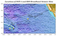
Figure 1. Locations are shown of Site 1224
and the Hawaii-2 Observatory (H2O) junction box (large star), Site 1223 (small
star), and the location of the Hawaii-2 cable (crosses). Superimposed on the
map is the satellite-derived bathymetry. Broadband seismometers have been installed
at the OSN1/843B and H2O/1224D sites. The Ocean Seismic Network site (OSN-1)
is 225km southwest of Oahu at a water depth of 4407m [Stephen et al., 2003].
The Hawaii-2 Observatory (H2O) is halfway between Hawaii and California on the
retired Hawaii-2 telecommunications cable and is at a water depth of 4970m.
Spectra from the two sites are compared in Figures 4 and
5.
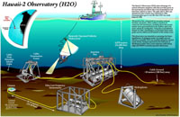
Figure 2. This artist’s conception
of the Hawaii-2 Observatory (H2O) summarizes some of the important components
of the installation (© copyright Jayne Doucette, Woods Hole Oceanographic
Institution [WHOI]. Reproduced with permission of WHOI).
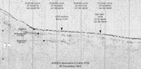
Figure 3. This 3.5kHz echo sounder recording
shows that the seafloor dips smoothly ~6m from the junction box to the drill
site (proposed Site H2O-5). One subbottom horizon at ~9m is fairly uniform throughout
the area. Based on drilling results, this is a mid sediment reflector. A second
reflector at ~30m below the junction box can be associated with basaltic basement
although it appears only occasionally in the record. PDR = precision depth recorder.
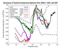
Figure 4. Vertical component spectra from
the seafloor, buried, and borehole installations at the Ocean Seismic Network
site (OSN-1) are compared with the spectra from the buried installation at the
Hawaii-2 Observatory (H2O) and from the Kipapa, Hawaii (KIP), Global Seismograph
Network station on Oahu. The H2O site has comparable noise levels to the OSN
seafloor and shallow buried stations near and above the microseism peak. Below
50mHz the noise levels of the buried sensor at H2O are comparable to the seafloor
sensor at OSN-1. The sediment resonances in the H2O spectrum near 1.1 and 2.3Hz
are prominent. The peak near 0.2Hz may also be effected by sediment resonances.
We would expect these to decrease substantially for a borehole sensor.
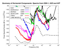
Figure 5. Horizontal component spectra
from the seafloor, buried, and borehole installations at the Ocean Seismic Network
site (OSN-1) are compared to the spectra from the buried installation at the
Hawaii-2 Observatory (H2O) and from the Kipapa, Hawaii (KIP), Global Seismic
Network station on Oahu. The sediment resonance peaks in the band 0.3 to 8Hz
are up to 35dB louder than background levels and far exceed the microseism peak
at 0.1 to 0.3Hz. That the resonance peaks are considerably higher for horizontal
components than for vertical components is consistent with the notion that these
are related to shear wave resonances (or Scholte modes).
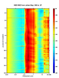
Figure 6. Spectrogram summary of ambient
noise levels on the vertical component of the Hawaii-2 Observatory (H2O) seafloor
Guralp seismometer for the duration of Leg 200. Color, as defined in the bar
on the right, indicates the relative energy content in decibels relative to
m/s^2 squared per hertz (from –190 to -90dB) as a function of frequency
from 0.001 to 60Hz. The broad red band at ~0.2–0.3 Hz throughout the week
is the microseism peak generated by wave-wave interaction of ocean gravity waves.
It appears to be modulated by sediment resonances. The thinner red band at 1.1Hz
and the yellow band at 2.0 Hz are resonances in the thin sediment cover at this
site. This spectrogram also shows storm cycles. These are the red bands that
slope upward to the left from ~1 to 0.2 Hz over 1.5 to 2 days for each storm
cycle. The high-energy peak at 8 Hz, on 25 December (Julian day 359), is a passing
ship (see Figure 14). The JOIDES Resolution arrived on
site at 1500hr on 26 December (Julian day 360). The patches of yellow from 4
to 9 Hz from 26 December to 20 January (Julian days 360/2001 to 20/2002) can
be associated with JOIDES Resolution activities (also see Figure
15).
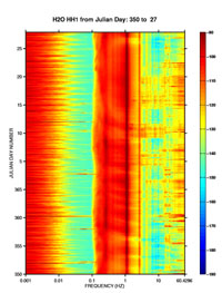
Figure 7. Spectrogram summary of ambient
noise levels on the horizontal component of the Hawaii-2 Observatory (H2O) seafloor
seismometer for the duration of Leg 200. Color, as defined in the bar on the
right, indicates the relative energy content in decibels relative to m/sec^2
squared per hertz as a function of frequency from 0.001 to 60Hz. By comparing
this horizontal component with the vertical component in Figure
6, one can see many more constant frequency bands. The main sediment resonances
near 1.1 and 2 Hz dominate even the microseism peak near 0.2 to 0.3 Hz.
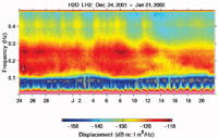
Figure 8. Horizontal component spectrograms
in the band 0.01-0.5Hz on one of the Guralp horizontals are shown for a 22day
window during the drilling on Leg 200. The peaks near 0.4Hz correlate with local
storm activity, while the 0.1-0.3Hz signals occur with the arrival of swell
from distant storms. The noise (increasing to the right) at long periods appears
to be caused by tidal currents.
Figure 9. Although no whales were seen
around the ship while on site, whale songs were frequently observed on the seafloor
seismometer. The largest-amplitude wavelets occur in wave packets of four, which
repeat about every 30 s. It takes this long for the water multiples to die down
to an acceptable level before the whale sings the next song.
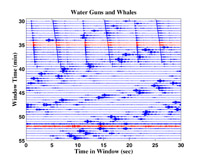
Figure 10. There is a similarity between
water guns and whale songs. The water guns are fired every 10 s in the top 10
min of this figure (30–40 s window time). The amplitude, frequency content,
and event interval are similar for the two sources. Note that no whale songs
are observed in the red traces ~15 min apart. In these intervals the whale stops
to breathe.
Figure 11. Tracking root-mean-square (RMS)
levels in one-octave bands is a convenient way to observe time-dependent effects
in the ambient noise data. The spikes around 5 and 20hr in this figure correspond
to earthquake events.
Figure 12. The top panel shows time series
near the earthquake at 21.3hr in Figure 11. The earthquake
occurs between 10 and 35s on the middle trace. The bottom panel shows the corresponding
color-coded power spectral density (PSD) in m/sec^2 squared per hertz. This
earthquake has shorter duration and a more uniform frequency content than the
event in Figure 13.
Figure 13. The top panel shows time series near the earthquake at 3.6hr in Figure 11. The earthquake occurs between 10 and 60s on the middle trace. The bottom panel shows the corresponding color-coded power spectral density (PSD) in counts squared per hertz. The microseism peak level is unchanged, but levels above the microseism peak increase by up to 20 dB. The events in Figures 12 and 13, which are observed on seismometers on the seafloor, have similar characteristics to the T-phases commonly observed on hydrophones in the ocean sound channel.
Figure 14. A container ship, with considerable energy above 4Hz, dominated the noise field near the sensor on 25 December. The ship starts raising noise levels at the site 6hr before its closest approach to the JOIDES Resolution, although it is ~180 km away (traveling at 17 kt). Root-mean-square (RMS) levels in octave bands are given in decibels relative to a m/sec^2.
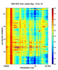
Figure 15. Horizontal component spectrograms in the band 2-20Hz are shown for a sequence of drilling and coring intervals. The quiet periods are when core was being recovered, and noisy times are when drilling core.
References
![]() Return to the Marine
Seismology and Geoacoustices Page
Return to the Marine
Seismology and Geoacoustices Page
Created December 9, 2003 by Tom Bolmer